Scarf's Economic Equilibrium Problem
Regularization via Auxiliary Term in General Equilibrium Models
Modified Equation using Auxiliary Term
Original Excess Demand: $F_i(x)$
1. Introduction
The computational algorithm for economic equilibrium problems developed by Herbert Scarf laid the foundation for Computable General Equilibrium (CGE) analysis and marked a significant milestone in the computer implementation of fixed-point theorems.
In this article, we address "Scarf's Example," a classic benchmark problem in general equilibrium theory. This problem presents a mathematical difficulty: simple iterative methods fail (the Jacobian matrix becomes singular) due to properties inherent in economic models.
We report on the results of introducing a special Auxiliary Term to regularize the equations and using the Homotopy Method to globally search for the solution.
2. Scarf's General Equilibrium Model
Consider a pure exchange economy with three commodities ($x_1, x_2, x_3$). Let $x = (x_1, x_2, x_3)$ be the price vector. The Excess Demand Function $F_i(x)$ in the market is defined as follows:
\[ \begin{cases} F_1(x) = \displaystyle \frac{x_3^\alpha}{x_1^\alpha + x_3^\alpha} - \frac{x_1^\alpha}{x_1^\alpha + x_2^\alpha} \\[10pt] F_2(x) = \displaystyle \frac{x_1^\alpha}{x_1^\alpha + x_2^\alpha} - \frac{x_2^\alpha}{x_2^\alpha + x_3^\alpha} \\[10pt] F_3(x) = \displaystyle \frac{x_2^\alpha}{x_2^\alpha + x_3^\alpha} - \frac{x_3^\alpha}{x_3^\alpha + x_1^\alpha} \end{cases} \]Here, $F_i(x) > 0$ indicates excess demand, and $F_i(x) < 0$ indicates excess supply. The goal is to find a price vector $x$ where the market clears, i.e., supply matches demand for all commodities ($F(x)=0$).
3. Mathematical Difficulties: Walras' Law and Rank Deficiency
Trying to solve this system of equations directly leads to computational failure. The reasons lie in two fundamental properties of general equilibrium models:
- Walras' Law:
The total value of excess demand is always zero ($\sum F_i(x) = 0$). This implies that the equations are not independent (one is redundant), causing the Jacobian matrix to become singular (rank deficient). - Homogeneity of Degree Zero:
Doubling all prices does not change the supply-demand balance ($F(kx) = F(x)$). Since the solution is indeterminate (infinitely many solutions exist), a normalization condition (e.g., $\sum x_i = 1$) must be imposed to uniquely determine the solution.
4. The Solution: Regularization via Auxiliary Term
To simultaneously solve the problems of "rank deficiency" and "normalization," we introduced the following Auxiliary Term into the equations.
We define a new function $G_i(x)$ by adding a term related to the sum of prices to all the original excess demand functions $F_i(x)$.
\[ G_i(x) = F_i(x) + \left( \sum_{j=1}^3 x_j - 1 \right) = 0 \]The added part, $\left( \sum x_j - 1 \right)$, is the auxiliary term.
Let's calculate the sum of the modified equations $\sum G_i(x)$. The original terms vanish due to Walras' Law ($\sum F_i = 0$), leaving only the auxiliary terms.
\[ \sum_{i=1}^3 G_i(x) = 0 + 3 \left( \sum x_j - 1 \right) \]Therefore, if we find a solution such that $G_i(x)=0$, it automatically implies $3(\sum x_j - 1) = 0$, meaning the normalization condition ($\sum x_j = 1$) is satisfied.
At the same time, since the auxiliary term itself becomes $0$, the original equations $F_i(x)=0$ also hold true.
5. Theoretical Prediction of the Solution
Before proceeding with numerical analysis, let us confirm the theoretically expected solution.
In this model (with $\alpha=1.0$), the equations are completely symmetric with respect to $x_1, x_2, x_3$. Therefore, the solution is also expected to be symmetric ($x_1=x_2=x_3$).
Since the auxiliary term imposes the condition "the sum equals 1" ($\sum x_i = 1$), the unique solution satisfying these conditions is:
\[ x_1 = x_2 = x_3 = \frac{1}{3} \approx 0.333... \]In the next section, we will perform the simulation to verify if the result converges to this value.
6. Analysis Results
Using the formulation described above, we traced the path from a trivial initial solution to the target equilibrium solution using the Fixed-point Homotopy Method. The homotopy method was implemented using the SPICE-oriented analysis method.
Trajectory of the Homotopy Path ($\alpha=1.0$)
The graphs of the simulation results are shown below.

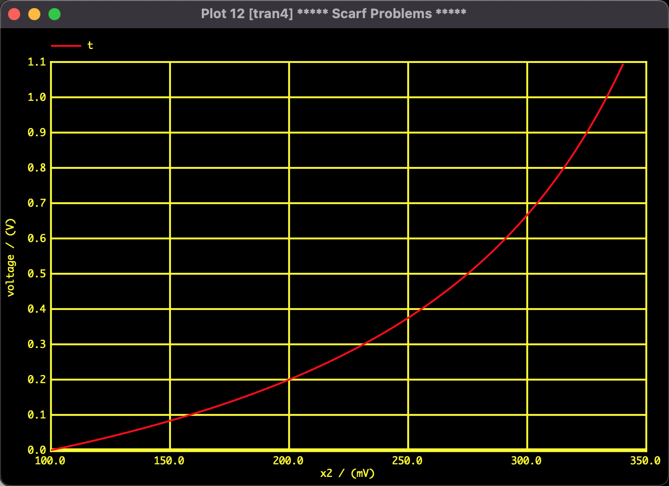
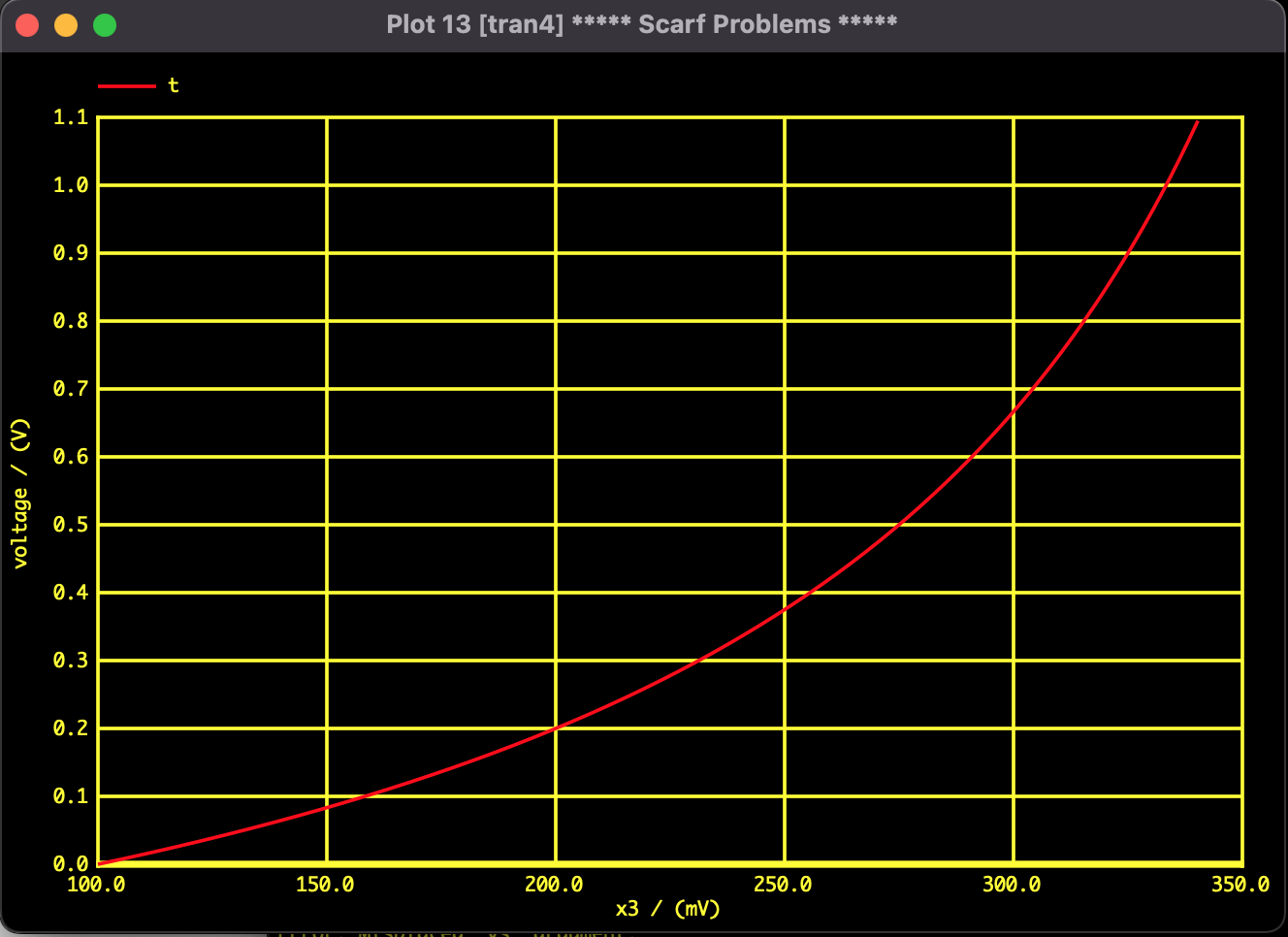
Starting from the initial state and advancing the parameter, the three variables converged smoothly.
The final arrival point is as follows:
$x_1 \approx 0.3333$
$x_2 \approx 0.3333$
$x_3 \approx 0.3333$
This result perfectly matches the theoretically predicted solution of $1/3$.
This demonstrates that the regularization method using the auxiliary term functioned correctly, avoiding the singularity caused by Walras' Law and successfully identifying the equilibrium prices.
Analysis Environment
- SPICE: Mac SPICE3
- PC: MacBook
- OS: macOS Monterey 12.7.6
- CPU: 1.2GHz Dual-Core Intel Core m5
- Memory: 8GB