Wilkinson's Polynomial

The "Monster" of Numerical Analysis and the Miracle of All-Solution Finding

$$W(x) = \prod_{i=1}^{20} (x - i) = (x-1)(x-2)\cdots(x-20) = 0$$

Wilkinson's Polynomial
Roots: $x = 1, 2, 3, \dots, 20$

1. Introduction: The Most Harmless-Looking Monster

Wilkinson's polynomial, introduced by James H. Wilkinson in 1959, is a classic example of an "ill-conditioned problem" in numerical analysis. Its roots are integers from $x = 1$ to $20$, and at first glance, it seems simple enough for a middle schooler to solve.

However, the moment you expand this equation to find its coefficients and feed it to a computer (floating-point arithmetic), it bares its fangs. By merely adding a microscopic noise of $2^{-23}$ (less than 1 bit in single-precision floating-point) to the coefficient of $x^{19}$ ($-210$), more than half of the real roots morph into complex numbers.

We dared to challenge this polynomial, which possesses an overwhelming vulnerability to round-off errors, using the Homotopy Method. We verified the results through three different approaches.

2. The Challenge via the Homotopy Method

This time, we implemented the Homotopy Method using M.A.L.'s core technology, the "SPICE-oriented approach", to search for the solutions.

① Newton's Method (Standard Solver)

Result: Solved (but local)

When running the standard Newton's method with an initial value (e.g., $x_0 = 0.1$), the massive gradient pushed it down to the nearest root, $x = 1$, where it converged. However, it only found this single solution.

② Fixed-Point Homotopy

Result: Defeat (Time step too small)

We formulated the following homotopy equation to find all solutions:
$$H(x,t) = t \cdot W(x) + (1-t)(x - x_0) = 0$$

The result: The transient analysis solver collapsed and stopped with an error. The cause was a "scale mismatch."
While the local maximum of $W(x)$ reaches about $10^{13}$, the penalty term $(x-x_0)$ is at most in the tens. This hopeless difference in dynamic range destroyed the Jacobian matrix, causing the simulator to shrink the time step to its limit before abandoning the calculation.

③ Newton Homotopy

Result: Victory (Successfully traced all 20 solutions)

Next, we reformulated the equation as follows:
$$H(x,t) = W(x) - (1-t)W(x_0) = 0$$

The simulation ran to completion without throwing any errors, drawing an incredibly beautiful trajectory and discovering all the solutions.

3. The Miracle of "Self-Scaling"

Why was only the Newton Homotopy method able to break through the limits of double-precision floating-point (double)?
The answer lies in the magic of "Self-Scaling" triggered by the structure of the equation itself.

Solving the equation for $t$, the trajectory of the path can be expressed as:
$$1 - t = \frac{W(x)}{W(x_0)}$$ Here, if we set the initial value $x_0 = 0.1$, the denominator $W(x_0)$ becomes an unimaginably massive value of approximately $2.4 \times 10^{18}$.

Even if the equation $W(x)$ wildly fluctuates up to about $10^{13}$ between roots, it is divided by a constant with an overwhelming scale of $10^{18}$. Thus, the fluctuation range of $t$ is perfectly confined to the order of $10^{-5}$ ($0.00001$).

By eliminating the distortion of "adding a small value to a massive value," the equation itself functions as a damper, allowing the Arc Length solver to proceed without losing its path.

4. Analysis Results: Astounding All-Solution Search

Below are the simulation results (trajectory in the $t - x$ plane) of the Newton Homotopy method implemented using the SPICE-oriented approach.

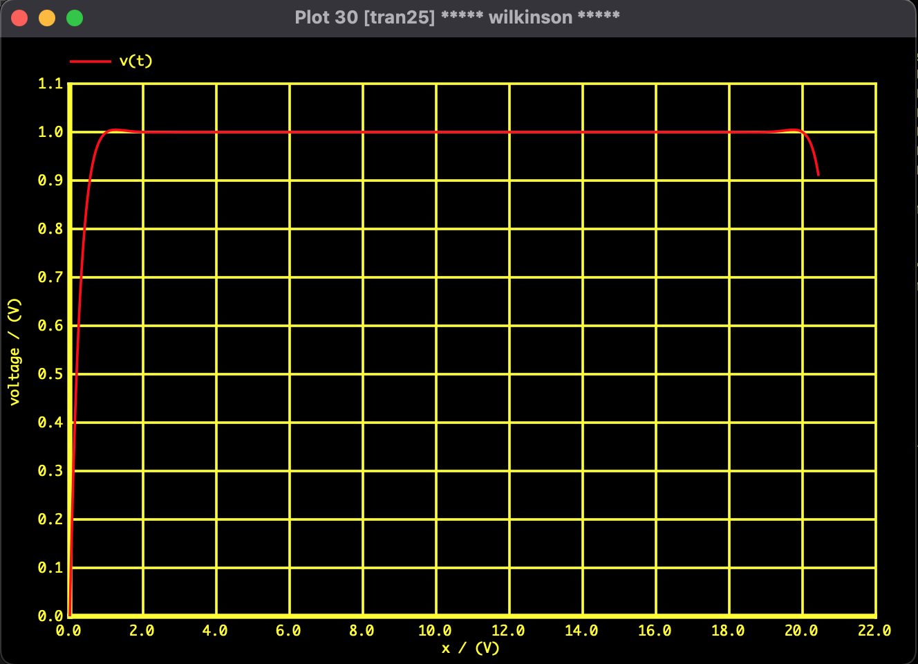
Graph: Wilkinson Polynomial Newton Homotopy Result 1

Fig 1: Overall view. While clinging to the $t=1.0$ line, $x$ appears to slide to the right.

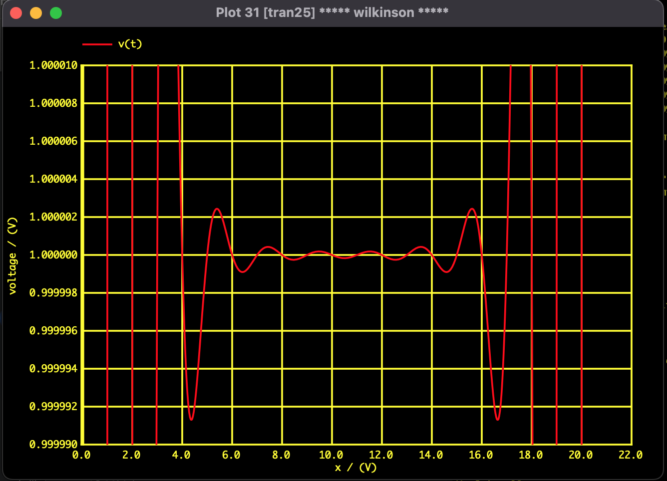
Graph: Wilkinson Polynomial Newton Homotopy Result 2 (Zoomed)

Fig 2: Enlarged view near $t=1.0$. Repeating microscopic oscillations, it pierces through all solutions from $x=1$ to $20$.

Dr.WataWata Insight：

Looking at the enlarged view (Fig. 2), the fluctuation of the vertical axis $t$ is beautifully contained between 0.999990 and 1.000010. The theoretical scaling of $10^{-5}$ is perfectly proven.

Even Wilkinson's polynomial, feared as an "ill-conditioned problem," can be beautifully tamed just by choosing the right algorithm (switching to Newton Homotopy).
Ascertaining both the mathematical properties and the numerical behavior of the solver (the scale of the Jacobian) simultaneously—this is the true thrill of mathematical engineering.

5. Analysis Environment

Analysis Engine: Mac SPICE3 (SPICE-oriented approach)
PC: MacBook
OS: macOS Monterey 12.7.6
CPU: 1.2GHz Dual-Core Intel Core m5
Memory: 8GB