Interior Point Method

Primal-Dual Path Following: Approaching the optimum along the Central Path

1. Introduction

While the Simplex Method explores the boundary (vertices) of the feasible region, the Interior Point Method traverses the interior of the region, following a "Central Path" to reach the optimal solution.

Since it outperforms the Simplex Method for large-scale linear programming problems, it is adopted in many modern mathematical optimization solvers. In this article, we explain the standard "Primal-Dual Path Following Method" in detail, from its mathematical derivation to specific numerical calculation procedures.

2. Mathematical Derivation

2.1 Primal and Dual Problems

Consider a standard Linear Programming problem and its Dual problem.

Primal (P):
Min $\boldsymbol{c}^T \boldsymbol{x}$
s.t. $\boldsymbol{Ax} = \boldsymbol{b}, \quad \boldsymbol{x} \ge 0$

Dual (D):
Max $\boldsymbol{b}^T \boldsymbol{y}$
s.t. $\boldsymbol{A}^T \boldsymbol{y} + \boldsymbol{s} = \boldsymbol{c}, \quad \boldsymbol{s} \ge 0$

2.2 Optimality Conditions (KKT Conditions)

The necessary and sufficient conditions for optimality are described by the KKT (Karush-Kuhn-Tucker) conditions:

$\boldsymbol{A x} - \boldsymbol{b} = \boldsymbol{0}$ (Primal Feasibility)
$\boldsymbol{A}^T \boldsymbol{y} + \boldsymbol{s} - \boldsymbol{c} = \boldsymbol{0}$ (Dual Feasibility)
$\boldsymbol{X S e} = \boldsymbol{0}$ (Complementarity: $x_i s_i = 0$)
$\boldsymbol{x} \ge 0, \ \boldsymbol{s} \ge 0$

* $\boldsymbol{X} = \text{diag}(x_1 \dots x_n)$, $\boldsymbol{S} = \text{diag}(s_1 \dots s_n)$, $\boldsymbol{e} = (1 \dots 1)^T$

2.3 Barrier Parameter and Central Path

In the Interior Point Method, instead of satisfying the complementarity condition $x_i s_i = 0$ directly, we relax it using a positive parameter $\mu$ (Barrier Parameter).

\[ x_i s_i = \mu \quad (\mu > 0) \]

The solution $(\boldsymbol{x}(\mu), \boldsymbol{y}(\mu), \boldsymbol{s}(\mu))$ to this system of equations traces a smooth curve called the Central Path. The algorithm tracks this path using Newton's method while gradually converging $\mu \to 0$.

2.4 Newton's Equation

To find the search direction $(\Delta \boldsymbol{x}, \Delta \boldsymbol{y}, \Delta \boldsymbol{s})$ from the current point $(\boldsymbol{x, y, s})$, we linearize the perturbed KKT conditions and solve the following large system of linear equations:

\[ \begin{bmatrix} \boldsymbol{A} & \boldsymbol{0} & \boldsymbol{0} \\ \boldsymbol{0} & \boldsymbol{A}^T & \boldsymbol{I} \\ \boldsymbol{S} & \boldsymbol{0} & \boldsymbol{X} \end{bmatrix} \begin{bmatrix} \Delta \boldsymbol{x} \\ \Delta \boldsymbol{y} \\ \Delta \boldsymbol{s} \end{bmatrix} = \begin{bmatrix} \boldsymbol{0} \\ \boldsymbol{0} \\ -\boldsymbol{X S e} + \mu \boldsymbol{e} \end{bmatrix} \]

3. Step-by-Step Calculation

To understand the theory, let's solve the same problem used in the Simplex Method page using the Interior Point Method.

Problem Setup (Converted to Minimization):
Min $-4x_1 - 3x_2$
s.t. $x_1 + x_2 \le 40, \quad 2x_1 + x_2 \le 60$

Introduce slack variables $x_3, x_4$ to convert to standard equality form.

\[ \boldsymbol{A} = \begin{pmatrix} 1 & 1 & 1 & 0 \\ 2 & 1 & 0 & 1 \end{pmatrix}, \quad \boldsymbol{b} = \begin{pmatrix} 40 \\ 60 \end{pmatrix}, \quad \boldsymbol{c} = \begin{pmatrix} -4 \\ -3 \\ 0 \\ 0 \end{pmatrix} \]

Step 0: Initialization

Choose a strictly positive point (interior point) that satisfies the constraints.

Primal $\boldsymbol{x}^{(0)}$: $(10, 10, 20, 30)^T$
Dual $\boldsymbol{y}^{(0)}$: $(-2, -2)^T$ (Assumption)
Dual Slack $\boldsymbol{s}^{(0)}$: $\boldsymbol{c} - \boldsymbol{A}^T \boldsymbol{y} = (2, 1, 2, 2)^T$ (All positive, OK)

Step 1: First Iteration

1. Calculate Gap and $\mu$
Current complementarity gap $\boldsymbol{x}^T \boldsymbol{s} = 10(2) + 10(1) + 20(2) + 30(2) = 130$
Current $\mu = 130 / 4 = 32.5$
Target $\mu_{target} = 0.5 \times 32.5 = 16.25$

2. Construct Newton's Equation ($10 \times 10$)
Solve the following system:

\[ \begin{bmatrix} 0 & 0 & 0 & 0 & 0 & 0 & 1 & 2 & 1 & 0 \\ 0 & 0 & 0 & 0 & 0 & 0 & 1 & 1 & 0 & 1 \\ 0 & 0 & 0 & 0 & 0 & 0 & 1 & 0 & 0 & 0 \\ 0 & 0 & 0 & 0 & 0 & 0 & 0 & 1 & 0 & 0 \\ 1 & 1 & 1 & 0 & 0 & 0 & 0 & 0 & 0 & 0 \\ 2 & 1 & 0 & 1 & 0 & 0 & 0 & 0 & 0 & 0 \\ 2 & 0 & 0 & 0 & 0 & 0 & 10 & 0 & 0 & 0 \\ 0 & 1 & 0 & 0 & 0 & 0 & 0 & 10 & 0 & 0 \\ 0 & 0 & 2 & 0 & 0 & 0 & 0 & 0 & 20 & 0 \\ 0 & 0 & 0 & 2 & 0 & 0 & 0 & 0 & 0 & 30 \end{bmatrix} \begin{bmatrix} \Delta \boldsymbol{x} \\ \Delta \boldsymbol{y} \\ \Delta \boldsymbol{s} \end{bmatrix} = \begin{bmatrix} 0 \\ 0 \\ 0 \\ 0 \\ 0 \\ 0 \\ -3.75 \\ 6.25 \\ -23.75 \\ -43.75 \end{bmatrix} \]

3. Solution and Update
Solving the equations gives the update vector:
$\Delta \boldsymbol{x} \approx (4.14, 1.76, -5.90, -10.04)^T$
The next point $\boldsymbol{x}^{(1)}$ becomes $(14.14, 11.76, \dots)$, confirming that we are advancing from the initial point $(10, 10)$ towards the optimal solution $(20, 20)$.

Convergence

Repeating this process reduces $\mu \to 0$, and the solution smoothly converges to the theoretical optimum $(20, 20)$.

4. Comparison with Simplex Method

Finally, let's compare the behavior of both algorithms.

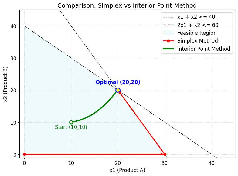
Trajectory Comparison: Simplex vs Interior Point

Fig 1. Trajectory Difference (Zigzagging Simplex vs Smooth Interior Point)

Feature	Simplex Method	Interior Point Method
Path	Moves along the Boundary (Vertices)	Moves through the Interior (Central Path)
Core Calculation	Pivot Operation (Basis Exchange)	Newton's Method (Large Linear System)
Strength	Medium-scale, when exact solution is needed	Very Large-scale problems (>10k variables)