Chandrasekhar's H-equation

Solving Integral Equations via SPICE

\[ H(\mu) = 1 + c \mu H(\mu) \int_0^1 \frac{H(\mu')}{\mu + \mu'} d\mu' \]

Unknown function: $H(\mu)$
Parameter: $c$ (Albedo, $0 \le c \le 1$)

Overview

In order to test the capabilities of the circuit simulator "SPICE" as a powerful "nonlinear equation solver," I attempted to solve the famous integral equation "Chandrasekhar's H-equation" appearing in astrophysics (radiative transfer theory).

Note: $\mu'$ (mu prime) is not a derivative
Although $\mu$ and $\mu'$ appear in the equation, this prime symbol ($'$) does not represent a derivative.

$\mu$: The specific direction for which we are currently calculating the value. Treated as a constant.
$\mu'$: Another direction variable that changes from $0$ to $1$ for the integral calculation.

In programming terms, $\mu$ is like a function argument, while $\mu'$ is like a loop counter variable.

Discretization Process for SPICE Solution

To solve this equation on a computer (SPICE), it is necessary to convert the "integral" in the equation into a "finite sum" and write it down as a system of simultaneous equations.
Here, I will explain the derivation process step-by-step.

Step 1: The Target Integral Term

We focus on the integral term on the right side of the original Chandrasekhar H-equation. Let's denote this as $I(\mu)$. Our goal is to convert this $I(\mu)$ into a summation form $\sum$.

\[ I(\mu) = \int_0^1 \frac{H(\mu')}{\mu + \mu'} d\mu' \]

Step 2: Introduction of Gauss-Legendre Quadrature

We use the "Gauss-Legendre quadrature," a powerful method for numerical integration. This formula works like magic when the integration interval is $[-1, 1]$.

\[ \int_{-1}^{1} g(t) dt \approx \sum_{j=1}^N w'_j g(t_j) \]

($t_j$: Zeros/roots of the Legendre polynomial, $w'_j$: Corresponding weights)

However, the interval of our integral $I(\mu)$ is $[0, 1]$. Since the formula cannot be used as is, we perform a variable change.

Step 3: Variable Change (Interval Adjustment)

To map the integration interval $[0, 1]$ to $[-1, 1]$ where the formula is applicable, we replace the variable $\mu'$ with a new variable $t$.

\[ \mu' = \frac{1}{2}t + \frac{1}{2} \]

Differentiating this expression gives $d\mu' = \frac{1}{2} dt$. Substituting this into the original integral $I(\mu)$:

\[ \begin{aligned} I(\mu) &= \int_{\mu'=0}^{1} \frac{H(\mu')}{\mu + \mu'} d\mu' \\ &= \int_{t=-1}^{1} \frac{H\left(\frac{t+1}{2}\right)}{\mu + \left(\frac{t+1}{2}\right)} \cdot \underbrace{\frac{1}{2} dt}_{d\mu'} \end{aligned} \]

The integration interval is now $[-1, 1]$, and a conversion factor of $\frac{1}{2}$ has appeared at the end.

Step 4: Applying the Summation Formula

Now that the interval is $[-1, 1]$, we apply the Gauss quadrature formula to rewrite the integral $\int$ as a sum $\sum$.
Here, for simplicity, we define the original coordinates corresponding to the transformed coordinates $t_j$ as $\mu_j$.

\[ \begin{aligned} I(\mu) &\approx \sum_{j=1}^N w'_j \cdot \left( \frac{H(\mu_j)}{\mu + \mu_j} \cdot \frac{1}{2} \right) \\ &= \frac{1}{2} \sum_{j=1}^N \frac{w'_j H(\mu_j)}{\mu + \mu_j} \end{aligned} \]

We have brought the factor $\frac{1}{2}$ outside the sigma.

Step 5: Derivation of the Final System of Equations

Finally, we substitute the calculated $I(\mu)$ back into the original H-equation and replace the continuous variable $H(\mu)$ with the discrete variable $x_i$. This yields the final equation to be implemented in SPICE.

\[ x_i = 1 + \frac{c}{2} x_i \sum_{j=1}^N \frac{w'_j \mu_i x_j}{\mu_i + \mu_j} \quad (i=1, \dots, N) \]

With this, the complex integral equation has been converted into a system of simultaneous equations that can be calculated using only basic arithmetic operations.

Calculation of Quadrature Points (Python)

Calculating the "zeros of Legendre polynomials" by hand is difficult, but it can be done instantly using Python. The following code generated the $\mu_i$ and weights $w_i$ used in this simulation.

import numpy as np

# 1. Get zeros t and weights w_prime of Legendre polynomial (domain -1 to 1)
N = 100
t, w_prime = np.polynomial.legendre.legauss(N)

# 2. Convert to the current integral interval [0, 1]
# mu  : Variable corresponding to SPICE node voltage
# w   : Weight used for resistance calculation, etc. (multiplied by 0.5)
mu = 0.5 * t + 0.5 
w  = 0.5 * w_prime

print(f"x1   (min) = {mu[0]:.6f}")
print(f"x100 (max) = {mu[-1]:.6f}")

Analysis Results

To solve the nonlinear equation with 100 variables, I utilized SPICE's .DC analysis (DC Sweep). The solution is tracked while continuously changing the parameter $c$ from $0$ to $1.0$.

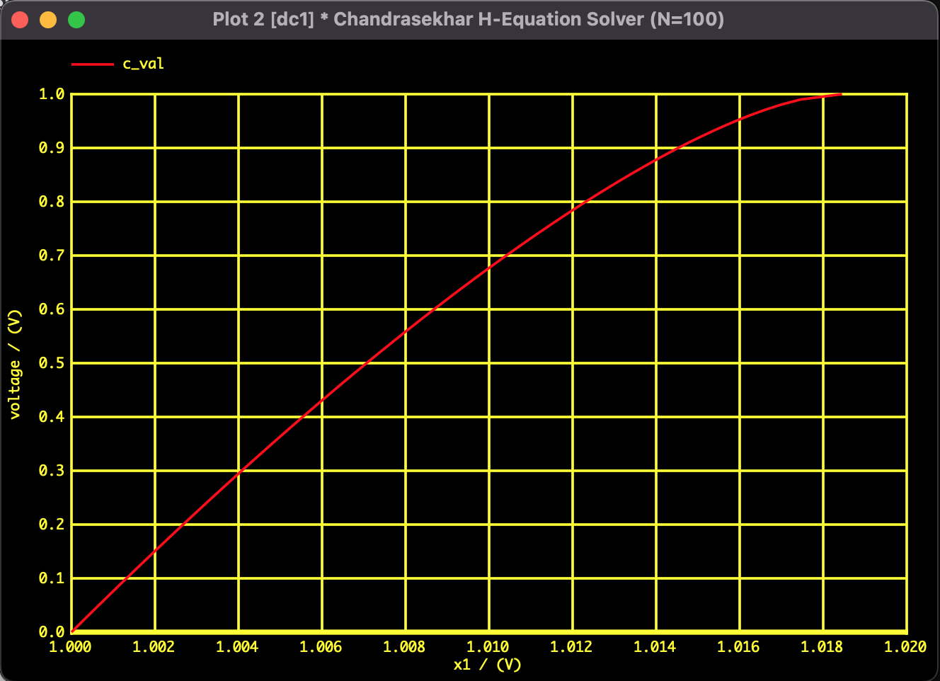
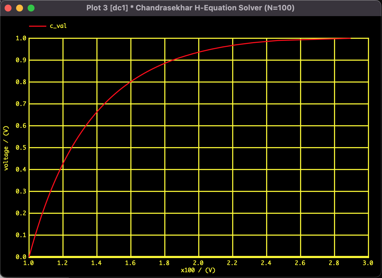
As a result of the simulation, the values at both ends ($x_1$ and $x_{100}$) at $c=1.0$ were as follows:

Variable (Position of $\mu$)	SPICE Measured Value	Theoretical Value (Approx)	Verdict
$x_1$ ($\mu \approx 0$)	1.01845	1.018	Good
$x_{100}$ ($\mu \approx 1$)	2.89526	2.899	Good

Using the analog circuit simulator SPICE, I successfully solved a complex integral equation with 100 variables with an accuracy of about 0.1%.

Analysis Environment

SPICE: Mac SPICE3
PC: MacBook
OS: macOS Monterey 12.7.6
CPU: 1.2GHz Dual-Core Intel Core m5
Memory: 8GB

Since calculation of this scale completes instantly in the current PC environment, detailed measurement of calculation time is omitted.