1D Heat Equation
Numerical Solution of Partial Differential Equations
Introduction
"How does heat propagate if one end of a hot iron rod is continuously heated?"
To understand such heat transfer phenomena, physics employs a partial differential equation known as the Heat Equation.
While the notation may seem complex at first, converting this into a form computable by a machine (Finite Difference Equation) reveals a very simple world of addition and subtraction: "My temperature is determined by my neighbors."
This article explains the process of "discretizing" the heat equation and visualizes how the numerical values evolve over time.
From PDE to Finite Difference Equation (Derivation)
Computers cannot directly handle "infinitely small changes (derivatives)." Therefore, we divide time and space into a fine mesh (grid) and approximate derivatives as "differences over very short intervals." This is called Discretization (Finite Difference Method).
2.1 Discretization of Space and Time
First, we divide the domain into a grid.
- Space ($x$): Divide the rod into intervals of $\Delta x$. Location is indexed by $i$ ($x_i = i \cdot \Delta x$).
- Time ($t$): Advance time in steps of $\Delta t$. Time is indexed by $n$ ($t_n = n \cdot \Delta t$).
The goal is to create an equation that finds the temperature at the next time step ($u_i^{n+1}$) using data from the current time step ($n$).
2.2 Time Derivative (LHS Transformation)
The left-hand side, $\frac{\partial u}{\partial t}$, represents the rate of temperature change over time. This is approximated simply by subtracting the "current value" from the "future value" and dividing by the time step.
2.3 Spatial Curvature (RHS Transformation)
The right-hand side, $\frac{\partial^2 u}{\partial x^2}$, is the second derivative, representing the "rate of change of the slope" (curvature).
This is obtained by taking the difference between the "slope to the right" and the "slope to the left" and dividing by the distance $\Delta x$.
Step A: Find the Slope (1st Derivative)
Calculate the slope on the right and left sides centering on yourself (position $i$).
- Slope to Right: $\frac{u_{i+1} - u_i}{\Delta x}$
- Slope to Left: $\frac{u_i - u_{i-1}}{\Delta x}$
Step B: Find the Change in Slope (2nd Derivative)
Take the difference of these slopes and divide by $\Delta x$.
Simplifying this yields a very clean form:
2.4 Assembly and Completion
Equating the LHS and RHS and solving for the "future value ($u_i^{n+1}$)" gives us the Finite Difference Equation ready for programming.
where coefficient $r = \frac{\alpha \Delta t}{(\Delta x)^2}$
Physical Interpretation and Simulation
Let's interpret the derived equation: $u_{\text{new}} = u_{\text{current}} + r \times (u_{\text{left}} - 2u_{\text{current}} + u_{\text{right}})$.
The term in the parentheses acts as the difference between "the sum of neighbors" and "twice yourself."
- If you are lower than the "average of neighbors" $\rightarrow$ Value is positive (Temperature rises).
- If you are hotter than the "average of neighbors" $\rightarrow$ Value is negative (Temperature drops).
Mathematically, this represents a diffusion phenomenon where "temperature changes to blend in with the neighbors."
[Diagram] Interaction between 3 Points
The next temperature of "Self ($u_i$)" is determined by
the temperature difference with "Neighbors ($u_{i-1}, u_{i-1}$)".
Manual Calculation Example
Let's trace the heat propagation with simple numbers.
(Coefficient $r = 0.5$, Left end fixed at 100, Initial values are 0)
t=1 (After 1 step):
2nd Point: 0 + 0.5 * (100 - 0 + 0) = 50
Result: [ 100, 50, 0, 0, 0 ]
t=2 (After 2 steps):
2nd Point: 50 + 0.5 * (100 - 100 + 0) = 50
3rd Point: 0 + 0.5 * (50 - 0 + 0) = 25
Result: [ 100, 50, 25, 0, 0 ]
By simply repeating this calculation, we can simulate how heat gradually propagates from left to right, forming a gradient.
Results
Here are the results of the analysis of the derived finite difference equation. Instead of writing a loop process in a programming language directly, we used a "SPICE-Oriented Analysis Method" where the PDE is solved by the circuit simulator SPICE.
SPICE Implementation (Semi-discretization / Method of Lines)
The equation described in the SPICE B-source differs from the finite difference equation in the previous section; it discretizes only space while keeping time continuous (differential).
Since this represents the "rate of change (current)," the time step $\Delta t$ is not included here. The internal capacitor in SPICE handles the integration in continuous time.
The coefficient here (SPICE parameter COEFF) is $\frac{\alpha}{(\Delta x)^2}$. (Note the absence of $\Delta t$!)
The calculation was performed with a spatial mesh number N=5.
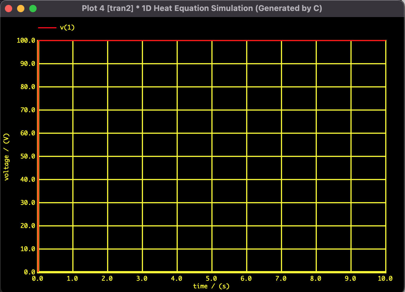
Fig 1: Time evolution of temperature distribution. The left end (Node 1) is fixed at 100V (°C). Over time, heat diffuses to the right, eventually converging to a linear temperature gradient (steady state).
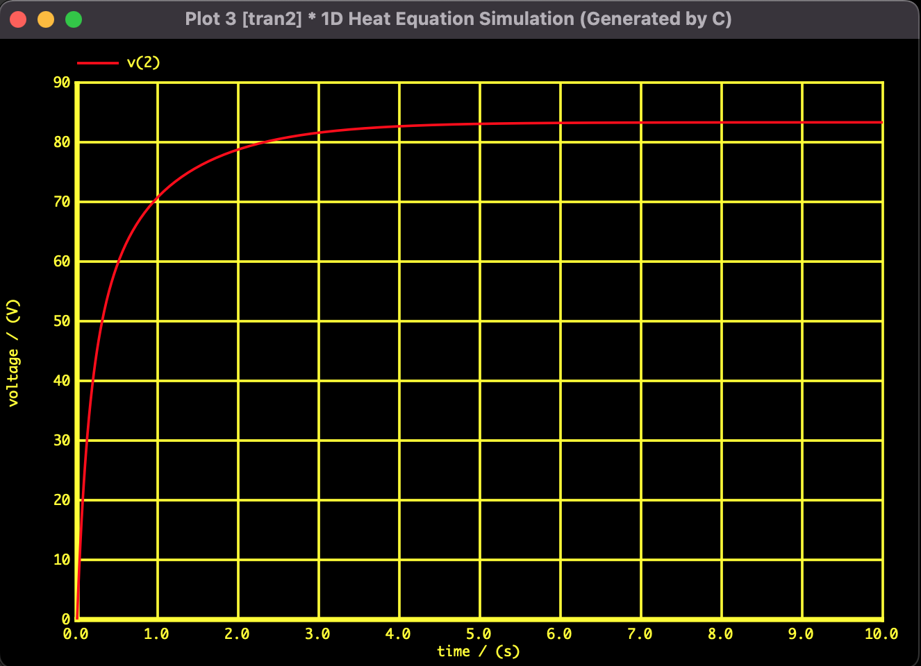
Fig 2: Transient response of a specific node (Node 2: The first division point from the left). It rises sharply at $t=0$ and converges to approximately 83.3V (theoretical value) like a first-order lag system. The solution is stable without divergence.
Simulation Environment
- Solver: Mac SPICE3
- Netlist Gen: C language (gcc)
- System: MacBook (macOS 12.7.6)
- CPU: 1.2GHz Dual-Core Intel Core m5
- Memory: 8GB
Since the calculation converges instantly in the current PC environment, detailed calculation time measurement is omitted.