Linear Programming

Klee-Minty Problem

1. What is Linear Programming?

Linear Programming (LP) is an optimization problem that maximizes (or minimizes) a linear objective function subject to linear equality or inequality constraints.

It is generally formulated in the following standard form:

\[ \begin{aligned} \text{Minimize} \quad & \boldsymbol{c}^T \boldsymbol{x} \\ \text{subject to} \quad & A\boldsymbol{x} = \boldsymbol{b} \\ & \boldsymbol{x} \ge 0 \end{aligned} \]

Where $\boldsymbol{x}$ is the decision variable vector, $A$ is the coefficient matrix, $\boldsymbol{b}$ is the constraint vector, and $\boldsymbol{c}$ is the cost vector.

While LP problems are typically solved using the Simplex Method or Interior Point Methods, this study approaches the problem as a dynamical system (energy minimization process) and explores the solution using continuous numerical analysis techniques.

2. The Klee-Minty Problem

We chose the "Klee-Minty problem," proposed by Klee and Minty in 1972, as the subject of our analysis.

This problem is known as a benchmark that forces the Simplex Method into its worst-case scenario (exponential time complexity) due to its feasible region, which resembles a distorted hypercube. Its geometry is extremely complex, characterized by numerous local traps and winding edges.

For $N$ variables, it is formulated as follows:

\[ \begin{aligned} \text{Maximize} \quad & \sum_{j=1}^{N} 10^{N-j} x_j \\ \text{subject to} \quad & 2 \sum_{j=1}^{i-1} 10^{i-j} x_j + x_i \le 100^{i-1} \quad (i=1, \dots, N) \\ & x_j \ge 0 \end{aligned} \]

Since the coefficients involve powers of 10, the scales of the variables differ strictly. This makes the problem computationally "ill-conditioned" for numerical analysis.

3. Augmented Lagrangian Method (Convex Formulation)

There are two main approaches to handling inequality constraints $g_i(\boldsymbol{x}) \le 0$.

(A) Equality Conversion using Slack Variables (Risk of Non-convexity)

A textbook approach is to introduce slack variables $y_i$ to convert inequalities into equalities $g_i(\boldsymbol{x}) + y_i^2 = 0$, and then construct the Augmented Lagrangian function.

\[ L(\boldsymbol{x}, \boldsymbol{y}, \boldsymbol{\lambda}) = f(\boldsymbol{x}) + \sum \lambda_i (g_i(\boldsymbol{x}) + y_i^2) + \frac{\rho}{2} \sum (g_i(\boldsymbol{x}) + y_i^2)^2 \]

However, since this method includes the $y_i^2$ term, the entire energy function becomes non-convex even if the original problem is convex. Consequently, in complex landscapes like the Klee-Minty problem, the solver easily falls into local minima and fails to reach the correct solution.

(B) Inequality Formulation by Rockafellar (Preserving Convexity)

Therefore, in this analysis, we adopted Rockafellar's formulation (Eq. 1.30), which handles inequality constraints directly without slack variables. This method forms a potential like a "one-sided spring" that applies a penalty only when constraints are violated, allowing convergence to the global optimum while maintaining convexity.

[Basic Equation]

\[ L(\boldsymbol{x}, \boldsymbol{\lambda}, \kappa) = f(\boldsymbol{x}) + \frac{\kappa}{2} \sum \left( [g_i(\boldsymbol{x})]_{-} \right)^2 + \sum \lambda_i [g_i(\boldsymbol{x})]_{-} \]

Definition: $[g_i(\boldsymbol{x})]_{-} = \min \{ -\frac{\lambda_i}{\kappa}, \ g_i(\boldsymbol{x}) \}$

Through completing the square, the above equation reduces to a simple form suitable for implementation (an expression with a ReLU-like rectification effect):

[Implementation Form]

\[ L \approx f(\boldsymbol{x}) + \frac{1}{2\kappa} \sum \left[ \min \left( 0, \ \kappa g_i(\boldsymbol{x}) + \lambda_i \right) \right]^2 \]

4. Nonlinear Equation Formulation (KKT Conditions)

Another approach to solving optimization problems is to formulate the KKT (Karush-Kuhn-Tucker) conditions—the necessary and sufficient conditions for optimality—and solve them as a system of nonlinear equations.

The KKT conditions for linear programming are derived from the relationship between the Primal and Dual problems as follows:

Derivation from Primal and Dual Problems

First, consider the Primal Problem and its corresponding Dual Problem.

Primal (P): $\text{Min } \boldsymbol{c}^T \boldsymbol{x} \quad \text{s.t. } A\boldsymbol{x}=\boldsymbol{b}, \ \boldsymbol{x} \ge 0$

Dual (D): $\text{Max } \boldsymbol{b}^T \boldsymbol{y} \quad \text{s.t. } A^T \boldsymbol{y} + \boldsymbol{s} = \boldsymbol{c}, \ \boldsymbol{s} \ge 0$

At the optimal solution, constraints must be satisfied in both the Primal and Dual problems (Feasibility).

Primal Feasibility: $A\boldsymbol{x} = \boldsymbol{b}, \ \boldsymbol{x} \ge 0$
Dual Feasibility: $A^T \boldsymbol{y} + \boldsymbol{s} = \boldsymbol{c}, \ \boldsymbol{s} \ge 0$

Furthermore, by the Strong Duality Theorem, the minimum value of the primal problem equals the maximum value of the dual problem at the optimal solution (Duality Gap = 0).

$\boldsymbol{c}^T \boldsymbol{x} = \boldsymbol{b}^T \boldsymbol{y}$

Substituting $A\boldsymbol{x}=\boldsymbol{b}$ and $\boldsymbol{c} = A^T \boldsymbol{y} + \boldsymbol{s}$ and simplifying yields the following relationship:

$(A^T \boldsymbol{y} + \boldsymbol{s})^T \boldsymbol{x} = (A\boldsymbol{x})^T \boldsymbol{y} \iff \boldsymbol{y}^T A \boldsymbol{x} + \boldsymbol{s}^T \boldsymbol{x} = \boldsymbol{y}^T A \boldsymbol{x}$
$\therefore \boldsymbol{s}^T \boldsymbol{x} = 0$

Since $\boldsymbol{x} \ge 0$ and $\boldsymbol{s} \ge 0$, for the inner product to be zero, it must be that $x_i s_i = 0$ for each component. This is called the Complementarity Condition.

Summarizing these three conditions (Primal Constraints, Dual Constraints, Complementarity) gives us the system of equations (KKT System) to be solved:

\[ \begin{aligned} Ax &= b \\ A^T y + s &= c \\ X s &= 0 \quad (\text{or } X s = \mu) \\ (x, s) &\ge 0 \end{aligned} \]

5. Analysis Results

In this analysis, we addressed the Klee-Minty problem for $N=3$. The theoretical mathematical solutions (Exact Solutions) for verifying the numerical results are as follows:

Variable	Exact Solution ($N=3$)
$x_1$	0
$x_2$	0
$x_3$	10,000
Objective Value	10,000

1. Results: Augmented Lagrangian Method

These are the results using the convex formulation and the SPICE-Oriented Analysis Method. The objective function value decreases monotonically over time, and smooth convergence to the theoretical optimal solution is confirmed.

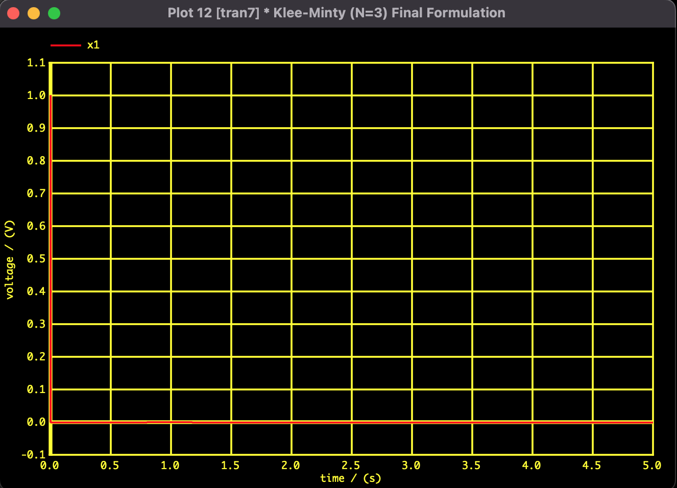
Fig 1: Convergence trajectory of $x_1$

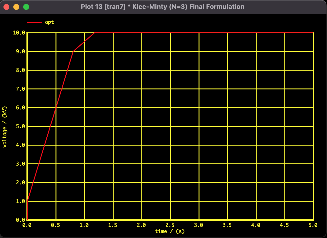
Fig 2: Convergence trajectory of Objective Function Value

2. Results: Newton's Method

We converted the Linear Programming problem into a system of nonlinear equations and applied a modified Newton's method using SPICE-Oriented Analysis. However, the solution did not converge.

During the line search from the initial value, the solver jumped over the constraints wall ($x \ge 0$) specific to the Klee-Minty problem and plunged into the negative region, stopping at an infeasible solution.

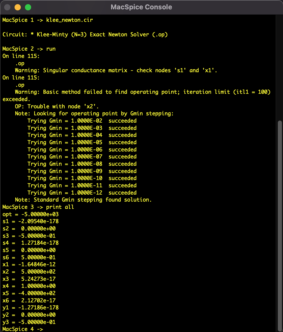
Fig 3: Analysis result of Newton's Method

3. Results: Homotopy Method

Following the failure of Newton's method, we applied the Homotopy Method, which introduces a parameter $t$ to continuously deform the equations.

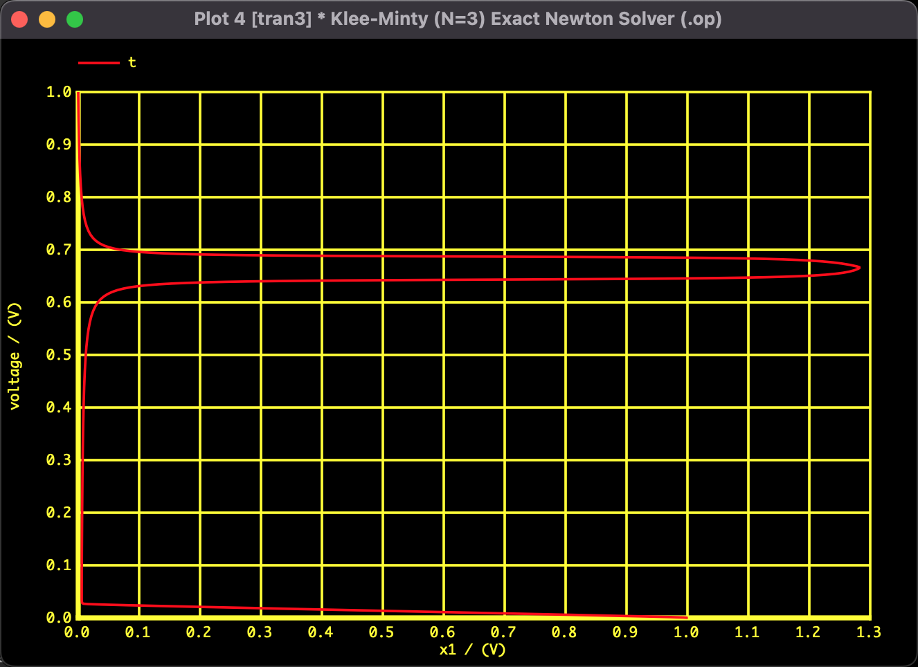
Fig 4: Solution path of $x_1$

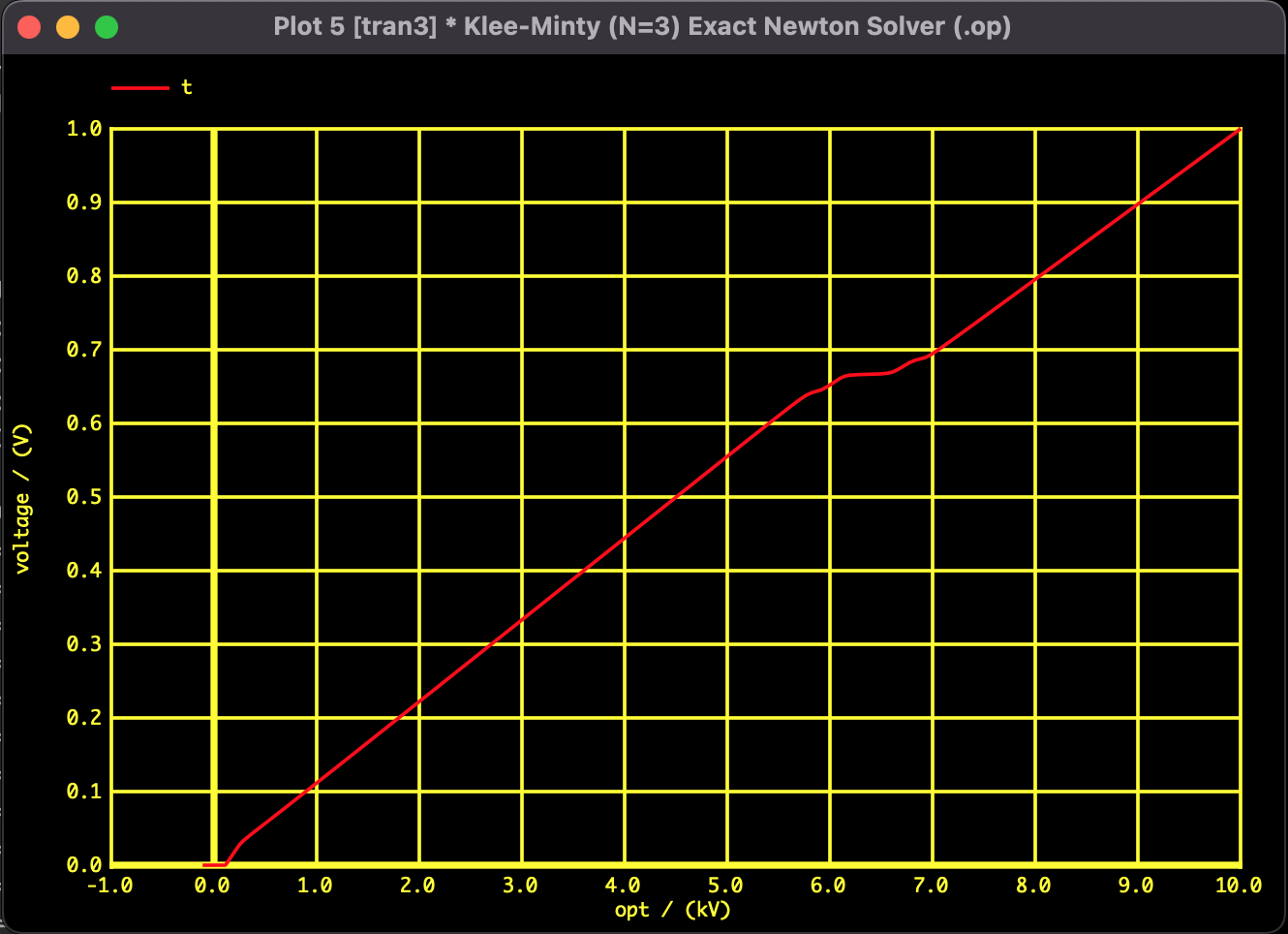
Fig 5: Convergence trajectory of Objective Function Value

The trajectory of $x_1$ is not a simple straight line but traces a large "S-curve." This visualizes how the solver navigates a route to the optimal solution, narrowly avoiding the constraint walls whenever it is about to collide with them.

Analysis Environment

SPICE: Mac SPICE3
PC: MacBook
OS: macOS Monterey 12.7.6
CPU: 1.2GHz Dual-Core Intel Core m5
RAM: 8GB

Since the calculation converges instantly on the current PC environment for this scale, detailed calculation time measurement is omitted.