Rosenbrock Function
01. Benchmark for Optimization
Characteristics
The Rosenbrock function is one of the most famous benchmarks for numerical optimization. By setting its gradient vector to zero, it is also frequently used as a test case for systems of non-linear algebraic equations.
The solution $(1, 1)$ lies at the bottom of a very narrow, curved valley. Because algorithms tend to slow down significantly as they approach the solution, it is ideal for evaluating convergence performance.
Solution Behavior
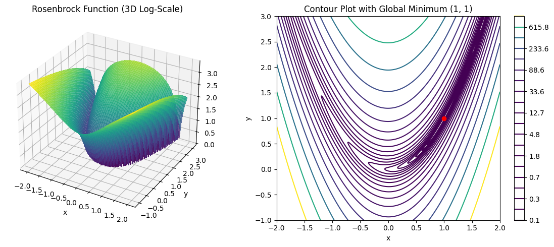
Fig 1: 3D surface plot of the Rosenbrock function. A very long and narrow valley is formed towards the solution at (1,1).
Results
The following shows the results of solving the Rosenbrock function using Newton's method.
Instead of conventional direct programming, the analysis was performed using the "SPICE-oriented approach," a methodology based on the unconventional idea of describing equations as electrical circuits and solving them with the SPICE circuit simulator.
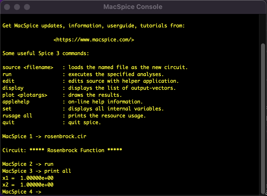
Fig 2: Analysis results of the Rosenbrock function using the SPICE-oriented approach.
Analysis Environment
- SPICE: Mac SPICE3
- PC: MacBook
- OS: macOS Monterey 12.7.6
- CPU: 1.2GHz Dual-Core Intel Core m5
- Memory: 8GB
Given the computational scale, convergence is achieved instantaneously on modern PC environments; therefore, detailed measurement of computation time has been omitted.