Numerical Integration for ODEs

Basics of ODEs and Stable Methods for Stiff Systems

1. Differential Equations and ODEs

A Differential Equation is an equation that describes the relationship between an unknown function and its derivatives (rate of change). Many dynamic laws in nature, such as equations of motion in physics or circuit equations in electrical engineering, are described in this form.

ODEs vs PDEs

Ordinary Differential Equation (ODE):
Involves only one independent variable (usually time $t$). Transient analysis in circuit simulation primarily deals with ODEs.
Partial Differential Equation (PDE):
Involves two or more independent variables (e.g., time $t$ and space $x, y, z$). These appear in electromagnetic field analysis or fluid dynamics.

General Form of an ODE

Letting the unknown function vector be $\boldsymbol{x}(t)$, a first-order ODE is generally expressed as:

\[ \frac{d\boldsymbol{x}}{dt} = \boldsymbol{f}(\boldsymbol{x}, t), \quad \boldsymbol{x}(t_0) = \boldsymbol{x}_0 \]

Here, $\boldsymbol{x}_0$ is the initial value. The goal of numerical analysis is to determine the sequence $\boldsymbol{x}_1, \boldsymbol{x}_2, \dots$ at each time step $h$ starting from this initial value.

2. The Stiff Problem

In circuit analysis, a system containing both extremely fast (small time constant) and slow (large time constant) components is called a Stiff equation.

With general explicit methods (such as Forward Euler or Runge-Kutta), the time step $h$ must be made extremely small to track the fastest changes in the system, causing computation time to explode. This is resolved by using Implicit Methods introduced below.

3. Trapezoidal Method

A second-order implicit method that estimates the next step using the average of the derivatives.

\[ \boldsymbol{x}_{n+1} = \boldsymbol{x}_n + \frac{h}{2} \left[ \boldsymbol{f}(\boldsymbol{x}_n, t_n) + \boldsymbol{f}(\boldsymbol{x}_{n+1}, t_{n+1}) \right] \]

Characteristics:

A-Stable: The calculation does not diverge anywhere in the left half of the complex plane.
Ringing: Due to weak damping characteristics, oscillation around the true value (Trapezoidal ringing) occurs at sharp transition points.

4. GEAR Method / Backward Differentiation Formula (BDF)

A multistep method that performs polynomial approximation using multiple past solution points. Proposed by C.W. Gear, it has become the standard method for circuit simulators.

\[ \boldsymbol{x}_{n+1} = \sum_{i=1}^{k} \alpha_i \boldsymbol{x}_{n+1-i} + h \beta_0 \boldsymbol{f}(\boldsymbol{x}_{n+1}, t_{n+1}) \]

Characteristics:

L-Stable: Rapidly dampens high-frequency components (eigenvalues at infinity), strongly suppressing numerical oscillation in stiff systems.
Order vs. Accuracy: Increasing the order $k$ improves accuracy, but creates a tradeoff with stability.

5. Stability Regions and Order Theory

The stability of numerical methods is evaluated by their absolute stability region on the complex plane.

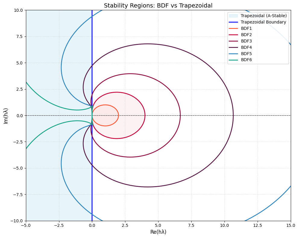
Stability Regions of BDF and Trapezoidal methods

Fig 1. Comparison of stability regions in the complex plane $h\lambda$

Important Note on Reading the Diagram (Interior vs Exterior):
Unlike explicit methods (such as Runge-Kutta), the stability region for implicit methods like BDF is the "Exterior" of the drawn boundary.

Trapezoidal: The entire left half-plane (Re < 0) is stable (A-Stable).
BDF 1-6: Everything outside the closed curves (unstable regions) is stable.

Dahlquist's Barrier

In the figure, for BDF orders of 3 and above, the unstable region (closed curve) protrudes into the left half-plane, indicating a loss of stability near the imaginary axis. This is a limit imposed by the mathematical theorem: "No multistep implicit method of order greater than 2 can be A-Stable."

Order	Stability	Application
1st (Backward Euler)	L-Stable (A-Stable)	Extremely stiff initial transient response
2nd (GEAR2 / Trapezoidal)	L-Stable / A-Stable	General-purpose simulation
3rd-6th (GEAR3-6)	Stiff Stable (Not A-Stable)	Systems requiring high precision but without extreme oscillatory components

6. Dr.WataWata's Insight

In the implementation of circuit simulators, numerical integration methods are not just formulas but engines that function in tandem with "Time-step Control" based on error estimation.

While the Trapezoidal method is suitable for analyzing oscillator circuits due to its energy conservation properties, the L-stable GEAR method (especially 2nd order) performs overwhelmingly well for systems requiring rapid decay, such as switching power supplies. Engineers are required not to rely solely on tools but to select the Method and Order according to the physical characteristics of the analysis target.