Double Pendulum
Chaos Theory and Conservation of Energy
Explanation: Chaos and Conservation Laws
A **Double Pendulum** is a physical system where a second pendulum is attached to the end of a first one. Despite its very simple structure, its behavior is extremely sensitive to initial conditions and is known as a classic example of unpredictable **'Chaos'**.
Verification via Energy Conservation Law
A crucial physical law in this system is the **'Law of Conservation of Mechanical Energy'**. In an ideal environment where friction and air resistance can be ignored, the sum $E$ of kinetic energy $K$ and potential energy $U$ must always remain constant, no matter how vigorously it moves.
In numerical simulation, the fact that this $E$ does not change over time is the strongest indicator guaranteeing calculation accuracy (reliability of the simulator).
Simulation and Governing Equations
In the demo below, you can observe the chaotic behavior when the initial position is set to horizontal ($\pi/2$).
The equations of motion (Lagrangian form) for a double pendulum with lengths $L_1, L_2$ and masses $m_1, m_2$ are as follows. We reproduce the movement above by numerically solving these coupled second-order nonlinear differential equations.
The following physical constants were used in this analysis:
- $m_1 = 1.0$ [kg], $m_2 = 1.0$ [kg]
- $L_1 = 1.0$ [m], $L_2 = 1.0$ [m]
- $g = 9.8$ [m/s$^2$]
Equations of Motion
Definitions
The relationship equations between velocity $\omega$ and angle $\theta$ (constraints in numerical integration) are as follows:
Results
Here are the results of the double pendulum analysis using the trapezoidal method.
In this instance, instead of direct programming, we performed the analysis using the **'SPICE-Oriented Analysis Method'**, a counter-intuitive methodology where equations are described as circuits and solved using the circuit simulator SPICE.
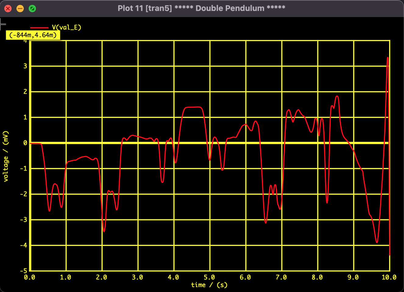
Fig 1: Correlation plot of $\theta_1$ and $\theta_2$ (Lissajous figure). Rather than simple periodic motion, a trajectory characteristic of chaos, which is complex and intertwined, can be confirmed.
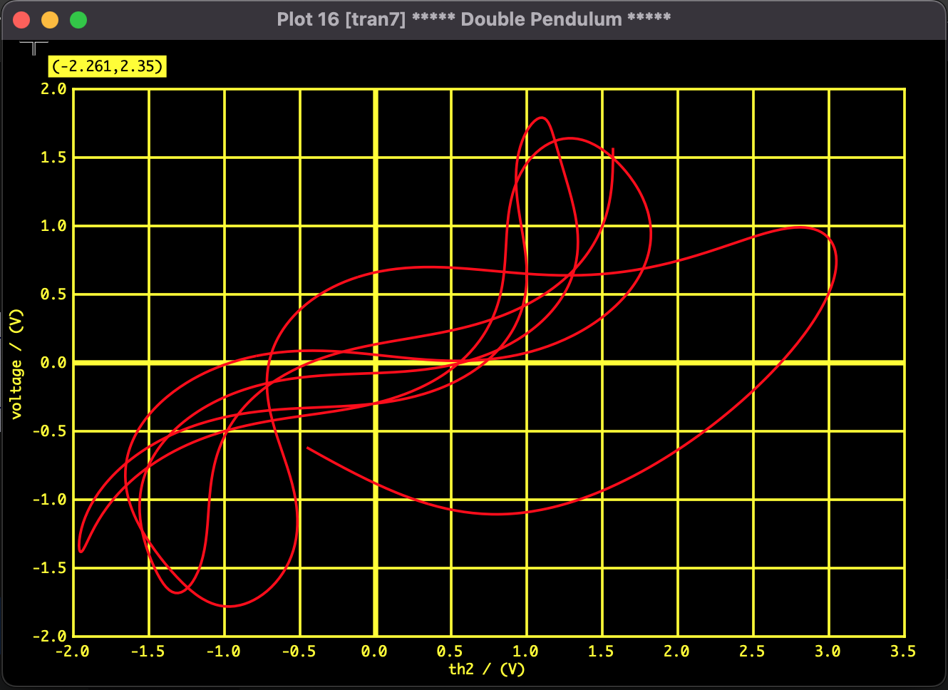
Fig 2: Time evolution of total energy. The unit of the vertical axis is [mV] (equivalent to millivolts/millijoules), and the error is kept within **0.01%** relative to the total energy scale (approx. 30J). This proves the high computational accuracy of this numerical analysis model.
Analysis Environment
- SPICE: Mac SPICE3
- PC: MacBook
- OS: macOS Monterey 12.7.6
- CPU: 1.2GHz Dual-Core Intel Core m5
- Memory: 8GB