Linear Complementarity Problem
LCP
1. What is the Linear Complementarity Problem (LCP)?
The Linear Complementarity Problem (LCP) is a problem of finding vectors $w$ and $z$ that satisfy specific conditions. It frequently appears in fields such as physics simulations (e.g., collision detection where rigid bodies must not penetrate each other) and economic equilibrium models.
The combination of the final "Complementarity Condition ($w^T z = 0$)" and the "Non-negativity Condition" implies a switching behavior: for each element, at least one of $w_i$ or $z_i$ must be zero, and neither can be negative.
2. General Methods and Our Approach
LCP has been studied for a long time, and several dedicated algorithms have been established to solve it.
- Pivot Methods (e.g., Lemke's Algorithm): Methods that search for a solution by swapping variables, similar to the Simplex method.
- Interior Point Methods: Methods that converge to the optimal solution through the interior of the feasible region.
However, in this study, we challenge ourselves to solve it using more general "Newton's Method" or "Homotopy Methods" instead of these dedicated solvers.
To do this, we need to reduce this problem involving inequalities ($\ge 0$) to a system of "nonlinear equations ($=0$)" that these powerful solvers can handle.
3. Reduction to Nonlinear Equations: NCP Functions
A function that can express the condition "non-negative and complementary ($a \ge 0, b \ge 0, ab=0$)" as a single equality $\phi(a, b) = 0$ is called an NCP function.
Here, we introduce two representative NCP functions.
A. Min Function (Using Absolute Values)
The most intuitive approach is the idea that "the smaller of the two must be zero."
If either is negative, the $\min$ is negative. If both are positive, the $\min$ is positive. It becomes zero only when "one is zero and the other is positive (or zero)," which is equivalent to the LCP condition.
Feature: While intuitive, it involves an absolute value, making the graph "kinked" (non-differentiable) at the line $a=b$. This is a disadvantage as it causes poor convergence for Newton's method.
B. Fischer-Burmeister Function (Main Focus)
To address this, we adopt the Fischer-Burmeister function, which uses a smooth curve instead of absolute values.
Why is it equivalent? (Proof)
Rearranging the equation and squaring it:
$\sqrt{a^2 + b^2} = a + b$
$\implies (a^2 + b^2) = (a + b)^2 = a^2 + 2ab + b^2$
$\implies 0 = 2ab \iff ab = 0$
This derives the condition "product is zero (at least one is zero)." Also, since the left side of the original equation (the root) is non-negative, the right side $a+b$ must also be non-negative. Combined with the product being zero, this inevitably implies $a, b \ge 0$.
Feature: It is smooth (differentiable) everywhere except at the origin, making it highly compatible with Newton's method. We will use this function.
4. Formulation of Equations
We apply the FB function $\phi_{FB}$ described above to each element of the vectors $(w_i, z_i)$.
Furthermore, by substituting the linear relation $w = Mz + q$ to eliminate $w$, we can create a system of simultaneous nonlinear equations with only unknown $z$.
With this, the LCP is reduced to a simple problem of solving $F(z)=0$.
5. Analysis Results
We set up the following parameters as a simple 2-dimensional example.
In this case, the linear relation $w = Mz + q$ becomes $w_i = -z_i + 1$, meaning $w = 1 - z$. Substituting this into the Fischer-Burmeister function $\phi_{FB}(w, z) = \sqrt{w^2 + z^2} - (w + z) = 0$, the actual equations to solve are:
* Since $(1-z_i) + z_i = 1$, the equation becomes very simple.
There are four solutions to this equation:
We verified whether all these solutions could be found using Newton's method and the Homotopy method. Note that this analysis was performed using SPICE-oriented analysis methods.
- (1) $z = (0, 0)^T$
- (2) $z = (1, 1)^T$
- (3) $z = (0, 1)^T$
- (4) $z = (1, 0)^T$
Result 1: Convergence using Newton's Method
This shows the convergence behavior when applying Newton's method with different initial values.

Figure 1: Convergence results of Newton's Method
Result 2: Search for solutions using Homotopy Method
We tracked the trajectory of the solution with parameter changes using the Newton Homotopy method. By changing the initial values, we could converge to different solutions and find all of them, but we were unable to find all solutions in a single analysis run.
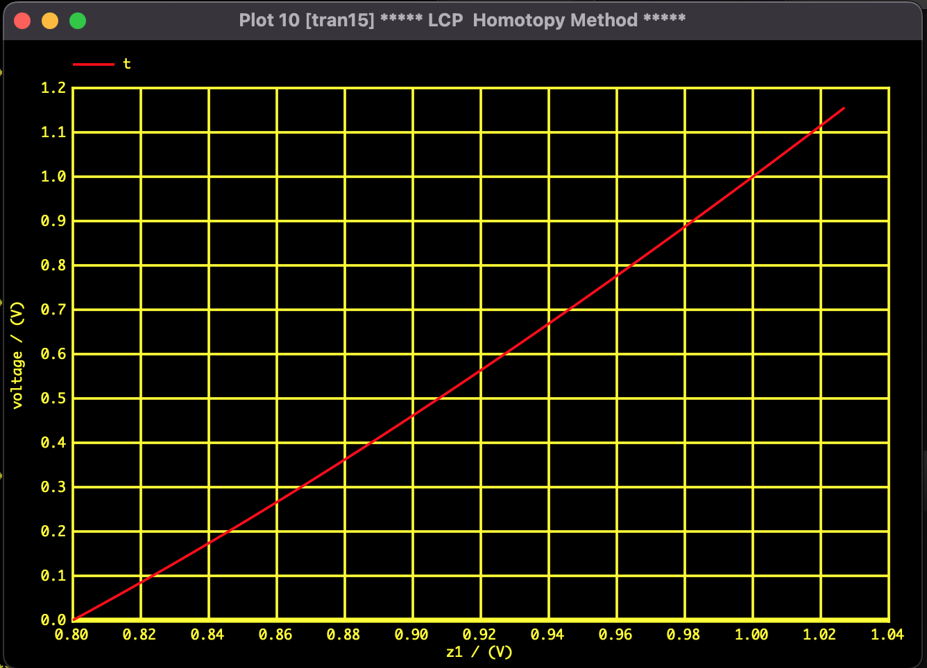
Figure 2: Trajectory of Homotopy Path ($z_1$)
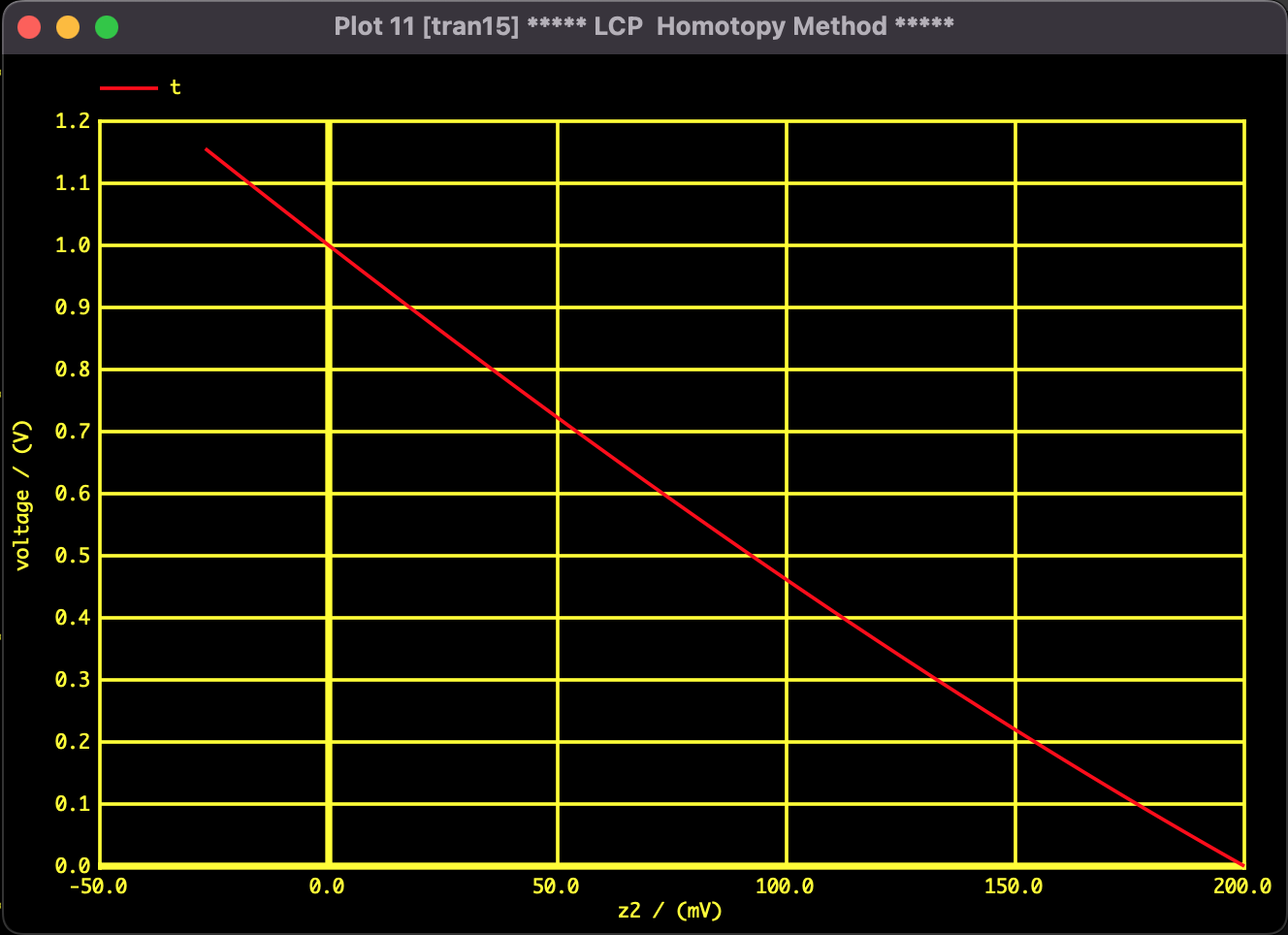
Figure 3: Trajectory of Homotopy Path ($z_2$)