Homotopy Global Search
The Challenge of Finding "All Solutions" via Homotopy Method
It is easy to find a single crow in the dark, but finding every crow there is an arduous task.
Discussing the difficulty of "Global Search" in nonlinear equations.
1. The Hard Problem of Finding "All Solutions"
When solving nonlinear algebraic equations $f(x)=0$, we typically use iterative methods like Newton's method. However, these methods depend heavily on initial values and terminate calculation once they converge to the nearest solution (local solution).
In real-world problems, such as chemical equilibrium or robot inverse kinematics, finding just "one solution" is often insufficient. To avoid missing physically meaningful solutions, it is necessary to exhaustively find "all solutions" existing in that space, which is considered a mathematically difficult task.
2. The 1972 Challenge: Branin's Benchmark
There are many benchmark problems for verifying global search algorithms, but one of the most interesting is the problem presented by F. H. Branin in his 1972 paper.
F. H. Branin, "Widely Convergent Method for Finding Multiple Solutions of Simultaneous Nonlinear Equations", IBM J. Res. Dev., 1972.
This paper deals with the gradient system equations of the so-called "Six-Hump Camel Function".
The difficulty of this problem lies in the number and arrangement of solutions. Combining local minima, maxima, and unstable saddle points, the total number of solutions is 15. These are scattered within a complicated terrain, and a simple search can only find a few of them.
3. Approach via Newton-Homotopy Method
To capture all 15 solutions in one fell swoop, I adopted the "Newton-Homotopy Method".
The Homotopy method does not attempt to solve the difficult problem $f(x)=0$ immediately. Instead, it starts from a simple problem $f(x_0)=0$ with a known answer and traces the trajectory of the solution while continuously deforming it.
$t$: Homotopy parameter ($0 \to 1$)
By changing the parameter $t$ from $0$ to $1$, a solution curve (path) is drawn in the space. By combining this with Branin's method (sign reversal of the determinant), it becomes possible to draw a single trajectory that visits all 15 solutions one after another, like beads on a string.
4. Experimental Results: A Journey Through 15 Solutions
The following shows the results of the search using the SPICE-oriented analysis method. In a single search, I successfully discovered all 15 solutions as theoretically predicted and completely reproduced the trajectory shown in Branin's paper.
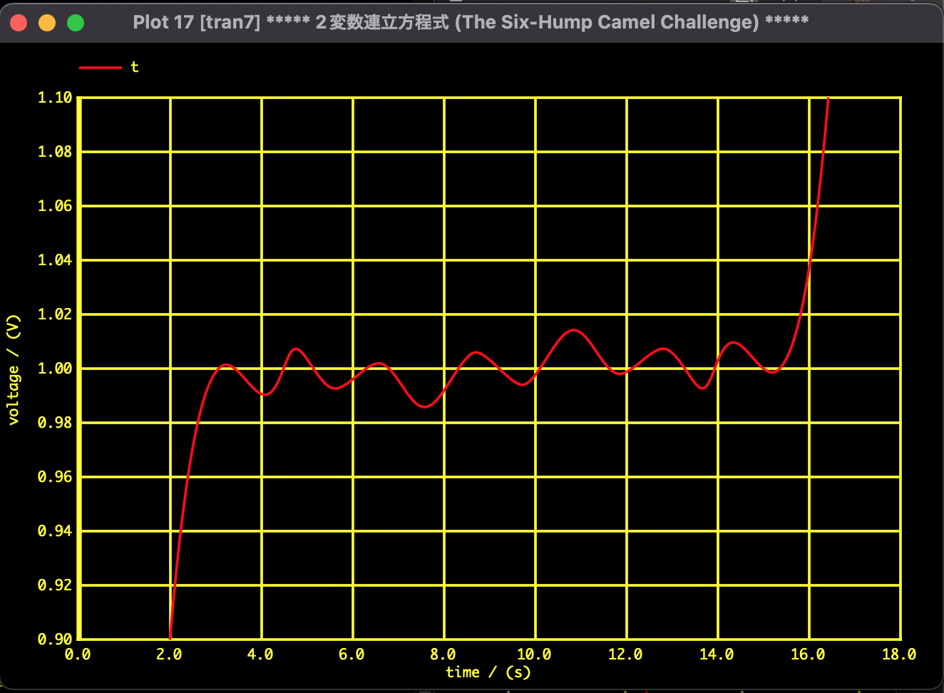
Fig.1: Horizontal axis: Time, Vertical axis: $t$. 15 solutions (maxima, minima, saddle points) connected by a single trajectory.
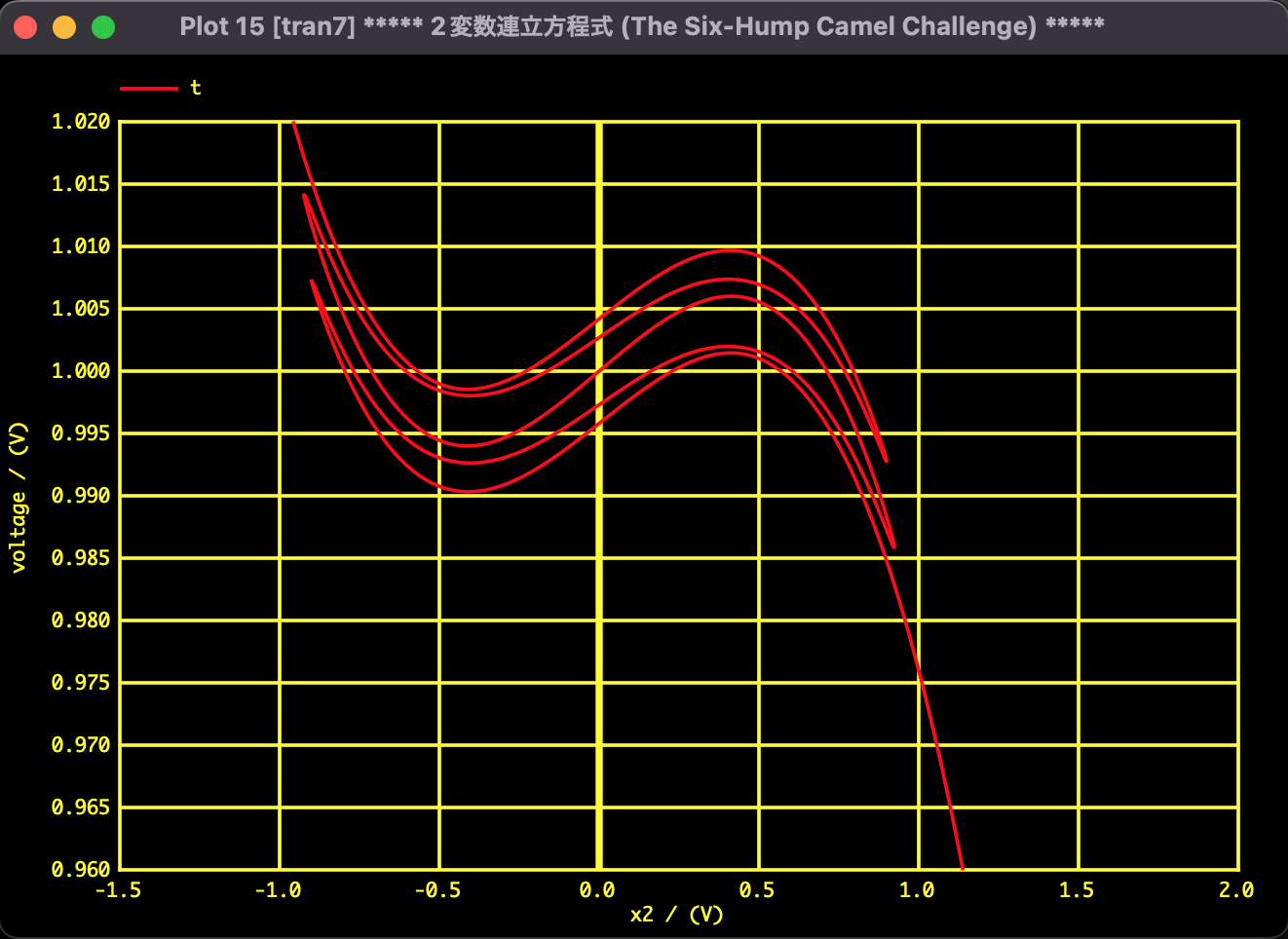
Fig.2: Horizontal axis: $x_1$, Vertical axis: $t$. Magnified view near solutions.
For the implementation of this complex nonlinear equation tracking, I did not use a general numerical calculation program (like C or Python), but used a unique attempt called "SPICE-Oriented Numerical Analysis Method".
This is a method of describing mathematical formulas as an electrical circuit netlist and diverting the robust transient analysis engine of a circuit simulator as a numerical solver. This enabled stable and high-precision tracking of the complex Homotopy trajectories.
5. Dr.WataWata's Insight
"The Answer Lies in Continuity"
Search methods that look for "points," like Newton's method, overlook isolated solutions. However, by rethinking the problem as a "line (continuum)" like in the Homotopy method, we can see that the 15 scattered solutions are actually connected by a single thread.
Events that seem unrelated at first glance become a single connected story by adding one parameter and raising the dimension. This perspective is highly suggestive not only in mathematics but also in our research and life.