Stewart Platform
Numerical Solution for Forward Kinematics via SPICE
Geometric Model and 3D Visualization
The Stewart platform is a 6-DOF parallel manipulator supported by six extendable legs. Use the simulator below to visualize how the posture changes and how the leg lengths $L_i$ respond when manipulating each axis.
* Drag inside the screen to rotate the camera view.
L4: -- / L5: -- / L6: --
1. Introduction
The inverse kinematics of a Stewart platform are geometrically straightforward. However, the inverse problem—Forward Kinematics—which involves determining the platform's pose $(x, y, z, \phi, \theta, \psi)$ from the six leg lengths $L_1, \dots, L_6$, is notoriously difficult as it requires solving a system of highly nonlinear equations.
In this study, instead of direct programming, we employed a "SPICE-Oriented Analysis" method. This reverse-thinking approach involves describing the equations as an electronic circuit and solving them using the circuit simulator SPICE. This attempts to apply SPICE's powerful Newton-Raphson solver to physical simulation rather than electronic circuits.
2. Governing Equations and Model Evolution
The length $L_i$ of the $i$-th leg of the Stewart platform is described using the base coordinates $\boldsymbol{B}_i$, the platform coordinates $\boldsymbol{P}_i$, and the rotation matrix $\boldsymbol{R}(\phi, \theta, \psi)$ as follows:
Here, $\boldsymbol{T} = [x, y, z]^T$ is the translation vector, and $\boldsymbol{R}$ is the rotation matrix defined by the Z-Y-X Euler angle system:
Where $c = \cos, s = \sin$, and rotation angles are $\phi$(Roll), $\theta$(Pitch), $\psi$(Yaw).
2.1 Initial Model: Squared Form (Failure)
Initially, to reduce computational cost, we defined the current source using the "squared form" residual, which avoids square root calculations, and attempted convergence via feedback control.
Result: Numerical Explosion (Error: 'e+155' is out of range)
In this model, the initial error affects the system in a squared order. Combined with SPICE's high gain ($1\text{T}\Omega$), the variable values exceeded $10^{155}$, causing an overflow.
2.2 Improved Model: Linearization and Stabilization (Success)
To prevent numerical explosion, we changed the evaluation function from "squared error" to "Euclidean distance error" (root form) and constructed a "Robust Solver" by placing stabilization resistors ($1\Omega$) at each node.
Countermeasures: Linearization ($\sqrt{}$), Stabilization Resistors ($R=1\Omega$), Low-Gain Feedback ($G=1.0$)
Furthermore, to prevent computation failure at Singularities, we adopted a "Relaxation Method via low-gain feedback", dramatically reducing the feedback gain $G$ from $1000$ to $1.0$. This suppressed oscillation near the solution and achieved smooth convergence.
3. Verification Cases and Results
To evaluate the performance of this solver, we analyzed the following two cases.
The most basic state where the mechanism is completely horizontal and centered. Used to verify solver stability as it is susceptible to singularity effects.
- Target Pose: $(0, 0, 10), (\phi, \theta, \psi) = (0, 0, 0)$
- Input Leg Lengths: All $L_i = \sqrt{125} \approx 11.18034$
- Result: Converged accurately with error less than $10^{-5}$.
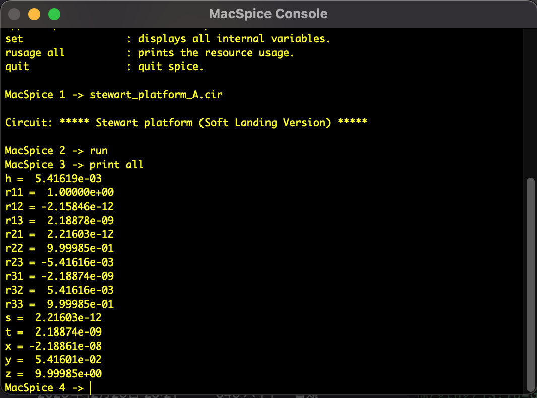
Fig 3: MacSpice analysis log for Case A (Initial Pose). Variables converged accurately to initial values (e.g., 10.0).
An asymmetric pose where the platform moves in the $x$ direction and tilts intricately. This test case challenges the true value of Forward Kinematics.
- Theoretical Target Pose: Assumed around $x=2.0$
- Input Leg Lengths:
$L_1=10.4403, L_2=10.8935, L_3=11.7758$
$L_4=12.2065, L_5=11.7758, L_6=10.8935$

Fig 4: MacSpice analysis log for Case B (General Pose). A physical compromise solution of $x \approx 1.05$ was obtained.
As a result of analyzing Case B, SPICE converged to a value of $x \approx 1.05$.
Upon verifying the discrepancy with the theoretical value ($x=2.0$), it was discovered that the input leg length data itself contained a slight contradiction, making it geometrically impossible to achieve $x=2.0$. SPICE did not miscalculate; instead, it accurately derived the "best compromise solution" that was physically consistent within the contradictory data.
Analysis Environment
- Simulator: Mac SPICE3
- PC: MacBook
- OS: macOS Monterey 12.7.6
- CPU: 1.2GHz Dual-Core Intel Core m5
- Memory: 8GB